Goal Programming

Goal programming (GP) is an extension of Linear Programming (LP). Essentially GP is LP with multiple objectives. The value of goal programming comes from a need optimize conflicting objectives which do not have a feasible solution, and where information to devise an accurate objective function is absent. In both of these cases, goal programming can be used to satisfy objectives as best as possible. Goal programming was first used by Dr. Cooper in 1955.

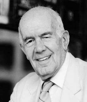
"Mr. Linear Programming": William W. Cooper (1914 - 2012)

Dr. Cooper was a busy man. It is hard to list all of the chapters he was a president of. For a bit of perspective, he received four honorary degrees: an M.A. from Harvard University in 1976, and honorary doctorates from Ohio State University in 1970, Carnegie Mellon in 1982, and the University of Alicante in 1995. Overall this man was a force to be reckoned with in the fields of Operations Research, Management Science, Business, and Accounting. With over 500 research articles and 27 books in his career, this man was the apotome of an expert.

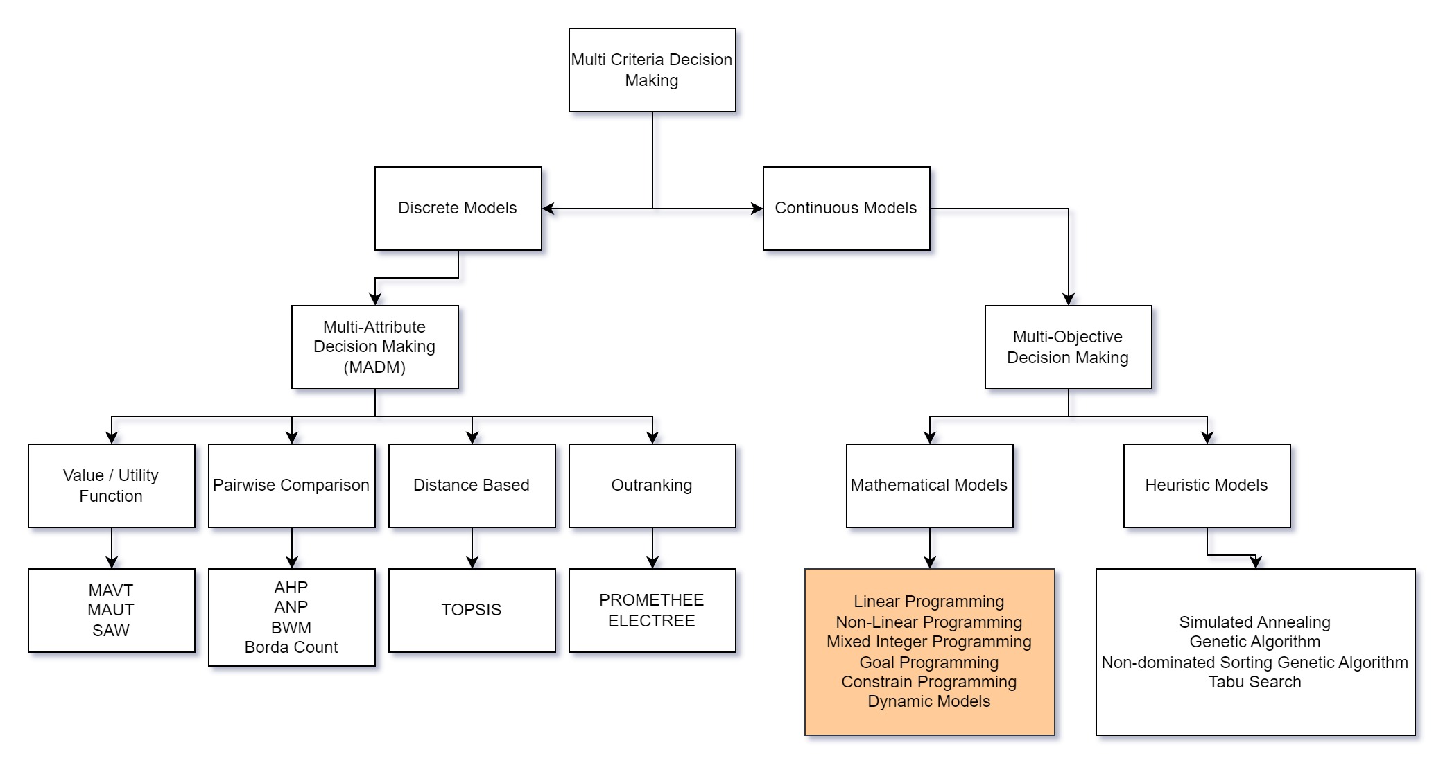
A map of *SOME* of the systems and acronyms in this field.

Brief Overview of Linear Programming

Lets take a step back. The foundation of GP is Linear Programming. LP problems seek to optimize some utility function which is bound by constraints.

Objective function: Defines how the decision variables $\vec{x}$ and cost variables $\vec{c}$ relate to the objective value $Z$.

$$ \text{max } Z = \sum_{j=1}^{n}{\vec{c}_{j} \vec{x}_{j}} $$

Constraints: Provide boundaries for the decision variables. $a_{ij}$ represents the resource requirement for the $i$-th resource and the $j$-th decision variable, and $b_i$ represents the boundary for that constraint.

$$ \text{subject to } \quad \sum_{j=1}^{n}{\textbf{a}_{ij} \vec{x}_{j}} \leq b_i \qquad \text{ for } i = 1,\dots,m$$

Variables: Here we set bounds for the variables themselves, for instance, we might want $x_j$ to always be positive

$$ \text{where } \quad \vec{x}_j \geq 0 \quad \text{for } j = 1, \dots, n $$

Example

Problem statement: Maximize profit by choosing how many stools and chairs to make.

Materials available:
- 75 square feet of wooden sheet (used for chair and stool seats, as well as chair backs).
- 100 wooden rods (used for chair and stool legs).
Materials consumed per product:
- chair consumes four wooden rods and four square feet of wood
- stool consumes three wooden rods (three legged stools...) and two square feet of wood.
Expected profit from the finished goods:
- $50 per chair
- $35 per stool

There are chairs and stools: $n$ = 2. Let $ x_1$ be the number of chairs to build and $ x_2$ the number of stools to build.

There are rods and wooden sheets: $m$ = 2. Let $i = 1$ represent the wooden sheet, and $i = 2$ represent the rods.

$$ \begin{aligned} \text{Maximize} \text{ Profit}\quad & = x_1 \cdot 50 + x_2 \cdot 35 \\ \text{Subject to} \quad & 4 \cdot x_1 + 2 \cdot x_2 \leq 75 \\ & 4 \cdot x_1 + 3 \cdot x_2 \leq 100 \\ \text{Where}\quad & x_1, x_2 \geq 0 \end{aligned} $$

There are three dominant vertices to the 2D solution space. One of these three vertices is the optimal solution. Like in many problems, integer values are troublesome. For simplicity, we can just round down each of these points and calculate the profit from each of them. This gives near optimal solutions.

Profit for each feasible edge solution

All Stools (0,33) = $1,155
Chairs and Stools (6,25) = $1,175
All Stools (0,33) = $900

Great! If we had a bigger problem or our results were more important, we could use the branch and bound method for solving an integer programming (IP) problem. Here I have implemented it in code:

# JuliaLang is very nice for solving optimization problems. 
using JuMP, HiGHS
# HiGHS is overkill for this but it works.
model = Model(HiGHS.Optimizer)

# We are initializing the variables as Integers.
# Technically this is not a Linear Programming problem.
@variable(model, x1 >= 0, Int)
@variable(model, x2 >= 0, Int)

# Setting constraint for the wooden sheet
@constraint(model, 4 * x1 + 2 * x2 <= 75)
# Setting the constraint for the rods
@constraint(model, 4 * x1 + 3 * x2 <= 100)

# Our objective function is to maximize this equation
# By changing x1 and x2, such that
# The constraints are still true.
@objective(model, Max, 50 * x1 + 35 * x2)

# Use the branch-and-bound technique to solve this IP
optimize!(model)

# Getting the saved values from the model
x1_opt = value(x1)
x2_opt = value(x2)
optimal_profit = objective_value(model)

println("Optimal x1: ", x1_opt)             #  x_1    = 4
println("Optimal x2: ", x2_opt)             #  x_2    = 28
println("Optimal profit: ", optimal_profit) #  Profit = $1,180

The actual optimal solution is the closest integer point to the LP solution which also happens to be an intercept of the two constraints.

Intro to Goal Programming

While there are two methodologies to Goal Programming, we will only be practicing one.

Preemptive: Also known as lexicographical, Goals are ranked by their priorities. Goals at a higher priority are infinitely more important than another goal at a lower priority. The model is solved top down, with the highest ranked goal solved first.
Non-preemptive: Also known as weighted, all objectives are reduced to some common unit and "mashed" together to be solved as one system.

We will be focusing on the preemptive methodology. Both methods must have a decision maker choose which goals have priority, but the preemptive methodology is more communicative of this, and there isn't an issue of finding common units between uncommon objectives.

Goal programming shines when there is no feasible solution satisfying all of the goals. Typically it is employed when objectives are working against each other. Goals and constraints can both be used on GP. Our example problem below will show how constraints and objectives come together to make an infeasible problem which goal programming will "solve".

Sample Problem

Our sample problem is a mixture problem. Working with fluids is a nice way to not have to dance around integer values. And Factorio makes oil processing seem somehow fun.

A refinery blends two types of crude oil: Oil A and Oil B. The Refinery sells two types of Gasoline: Regular and Premium. The higher ups have decided that the priorities for oil production are ordered as follows:

(Primary): Produce at least 5000 gallons of Regular Gasoline.
(Secondary): Produce at least 3000 gallons of Premium Gasoline.
(Tertiary): Keep the cost of crude oil below $17,500.

Additionally, in order to sell the gas, the sulfur content must be below certain limits.

The following information is known:

Oil A costs $2.50 per gallon and contains 0.4% sulfur.
Oil B costs $3.50 per gallon and contains 0.8% sulfur.
Each gallon of Oil A contributes 0.7 gallons to Regular Gasoline and 0.3 gallons to Premium Gasoline.
Each gallon of Oil B contributes 0.5 gallons to Regular Gasoline and 0.5 gallons to Premium Gasoline.
The maximum allowable sulfur content in Regular Gasoline is 0.7%, and in Premium Gasoline is 0.5%.

As the decision maker, we want to say with some certainty what combination of Oil A and Oil B should be used to satisfy the objectives. Not all objectives will necessarily fit together neatly, some sacrifices will have to be made. While the solutions should try to attain all of the goals, there is no feasible solution which does so.

The goal programming equations look like this:

$$ \begin{aligned} \text{Maximize} \quad & something & \\ \text{Subject to} \quad & x_1 \cdot 0.7 + x_2 \cdot 0.3 \geq 5000 \\ \quad & x_1 \cdot 0.5 + x_2 \cdot 0.5 \geq 3000 \\ \quad & x_1 \cdot 2.5 + x_2 \cdot 3.5 \leq 17500\\ \quad & x_1 \cdot 0.004 \cdot 0.7 + x_2 \cdot 0.008 \cdot 0.5 \leq (x_1*0.7 + x_2 * 0.5) \cdot 0.007\\ \quad & x_1 \cdot 0.004 \cdot 0.3 + x_2 \cdot 0.008 \cdot 0.5 \leq (x_1*0.3 + x_2 * 0.5) \cdot 0.005\\ \text{Where}\quad & \vec{x}_1, \vec{x}_2 \geq 0 \end{aligned} $$

Instead of optimizing the actual objective function, we can optimize the deviations from an optimal solution. For each goal, we can write the inequality as an equality with deviations. this looks like:

$$ \begin{aligned} \text{Minimize } Z = \quad & d_1^{-} + d_2^{-} + d_3^{+}\\ \text{Subject to} \quad & x_1 \cdot 0.7 + x_2 \cdot 0.3 + d_1^{-} - d_1^{+} = 5000 \\ \quad & x_1 \cdot 0.5 + x_2 \cdot 0.5 + d_2^{-} - d_2^{+} = 3000 \\ \quad & x_1 \cdot 2.5 + x_2 \cdot 3.5 + d_3^{-} - d_3^{+} = 17500\\ \quad & -0.0021 \cdot x_1 + 0.0005 \cdot x_2 \leq 0 \\ \quad & -0.0003 \cdot x_1 + 0.0015 \cdot x_2 \leq 0\\ \text{Where}\quad & \vec{x}_1 ,\vec{x}_2 , d_1^{-}, d_1^{+} , d_2^{-}, d_2^{+} , d_3^{-}, d_3^{+} \geq 0 \end{aligned} $$

Note the deviation $d_1^{+}$ communicates the positive deviation (how much the LHS exceeds the RHS) in the first constraint, and $d_1^{-}$ communicates how much the RHS exceeds the LHS in the first constraint. When optimizing constraints with a $\geq$ equality, we want to minimize the $d_1^{-}$ so that the values are as close to the goal as possible. There is no value added in exceeding the goals. Sometimes analysts will include a penalty for not achieving goals, but it is not strictly necessary.

"Do it yourself"

Download Goal Programming Example

Familiarize yourself with the worksheet

Figure 1: This section restates the problem.

Figure 2: This section has the decision variables as well as the Rates and Costs for the problem.

Figure 3: This is the output of the model. Goal values and deviations are on the left, constraints are on the right.

We want to find values of $x_1$ and $x_2$ which satisfy our constraints and meet as many of the goals as possible. To do this, we will use the excel solver.

a) First we want to see if we can meet the first goal (regular gasoline) volume. We want to minimize deviations BELOW the target, as it is a $\geq$ constraint.

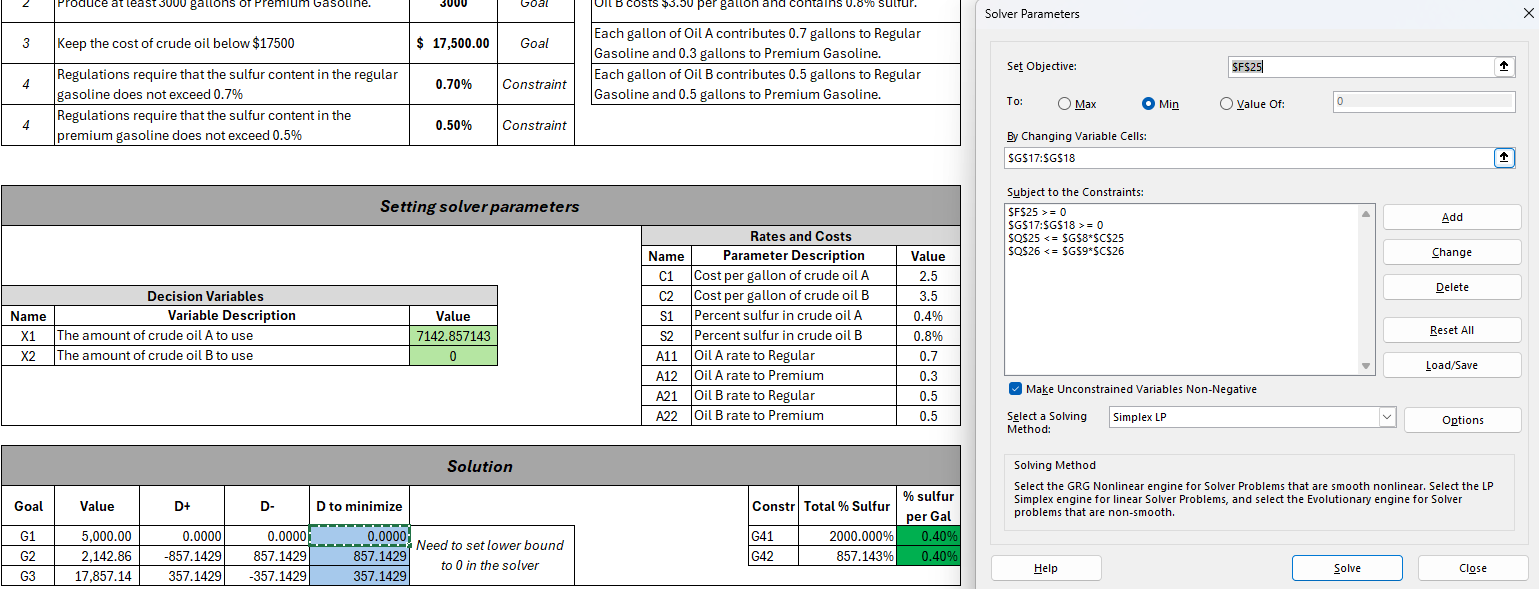Figure 4: Optimize the deviation for goal 1.

b) Next, we want to see if we can meet the second goal (premium gasoline) volume while maintaining our deviation of 0 for goal 1. We want to minimize deviations BELOW the target, as it is a $\geq$ constraint.

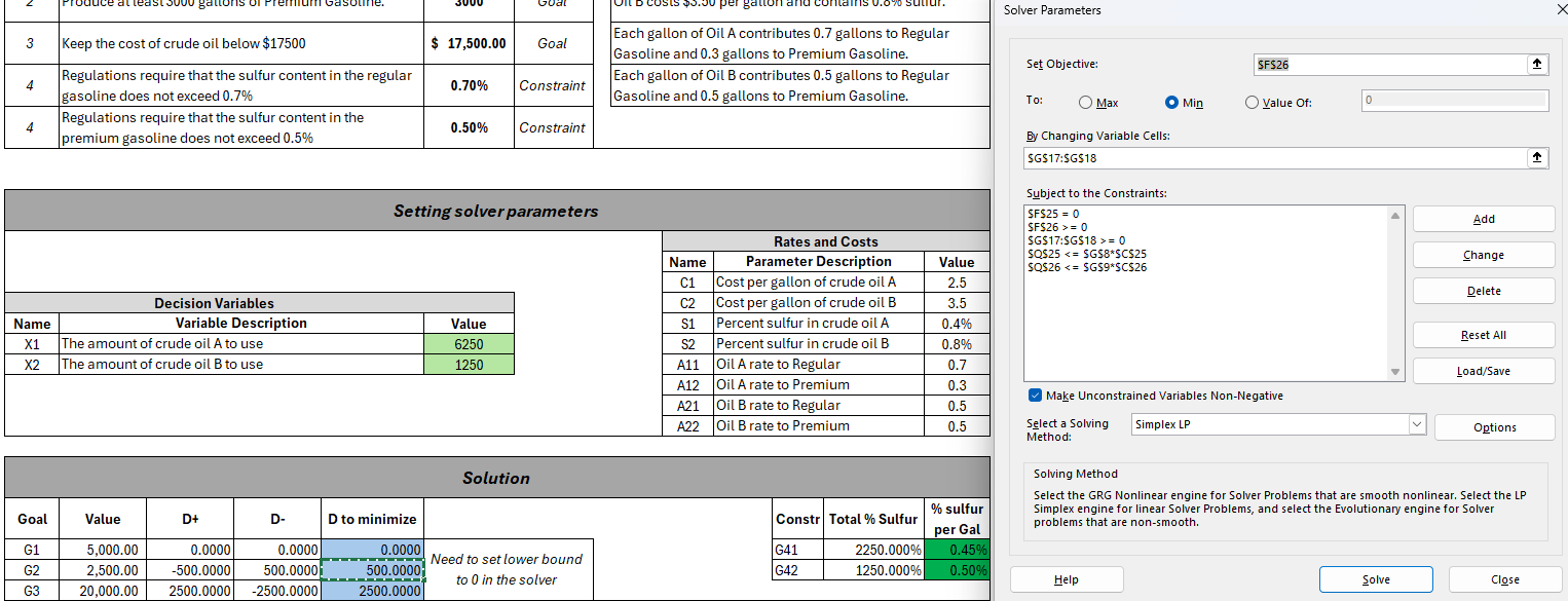Figure 5: Optimize the deviation for goal 2 while maintaining the deviation for goal 1.

c) Finally, we want to see if we can meet the third goal (cost of oil) while maintaining our deviation of 0 for goal 1, and 500 for goal 2. We want to minimize deviations ABOVE the target, as it is a $\leq$ constraint.

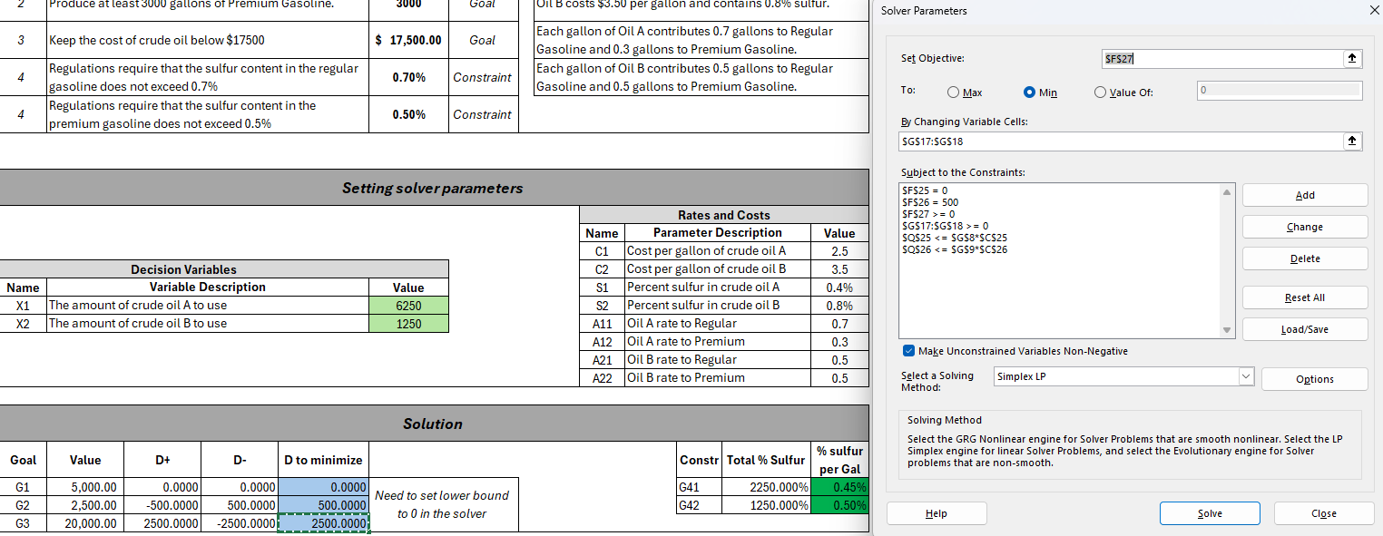Figure 6: Optimize the deviation for goal 3 while maintaining the deviations for goals 1 and 2.

Now we have the optimal lexicographical solution the for the decision values relative to the problem statement. We should use 6250 units of oil A and 1250 units of oil B. We do not attain goals 2 or 3. The sulfur concentration for premium gasoline is a bounding constraint; it has no slack. The sulfur concentration for regular gasoline has .25% of slack.

Discussion

What is good about this approach?
What is not good about this approach?
Should goals be revamped to become more feasible?
What if Oil A and Oil B had different rates or costs? Theoretically, how could we adjust them to be more feasible?

Bonus problem

Introduction

You work at an advertising agency. A customer has identified three primary target audiences they are trying to reach, and has an advertising budget of $600,000. They have expressed their targets in the form of three goals:

Ads should be seen by at least 40 million high-income men (HIM)
Ads should be seen by at least 50 million low-income people (LIP)
Ads should be seen by at least 35 million high-income women (HIW)

Type (per minute)	HIM	LIP	HIW	Cost
Football	7 million	10 million	5 million	$100,000
Soap Opera	3 million	5 million	4 million	$60,000

Formulate the Goals and Constraints for this problem

$$ \begin{aligned} \text{Goal } 1 \quad & 7 \cdot x_1 + 3 \cdot x_2 \geq 40 \\ \text{Goal } 2 \quad & 10 \cdot x_1 + 5 \cdot x_2 \geq 60 \\ \text{Goal } 3 \quad & 5 \cdot x_1 + 4 \cdot x_2 \geq 35 \\ \\ \text{Constraint } \quad & 100 \cdot x_1 + 60 \cdot x_2 \leq 600 \\ \\ \text{Where}\quad & x_1, x_2 \geq 0 \end{aligned} $$

Formulate System with deviations

$$ \begin{aligned} \text{Minimize} \quad & d_1^{-} + d_2^{-} + d_3^{-} \\ \text{Goal } 1 \quad & 7 \cdot x_1 + 3 \cdot x_2 + d_1^{-} - d_1^{+} = 40 \\ \text{Goal } 2 \quad & 10 \cdot x_1 + 5 \cdot x_2 + d_2^{-} - d_2^{+} = 60 \\ \text{Goal } 3 \quad & 5 \cdot x_1 + 4 \cdot x_2 + d_3^{-} - d_3^{+} = 35 \\ \\ \text{Constraint } \quad & 100 \cdot x_1 + 60 \cdot x_2 \leq 600 \\ \\ \text{Where}\quad & x_1, x_2, d_1^{-}, d_1^{+}, d_2^{-}, d_2^{+}, d_3^{-}, d_3^{+} \geq 0 \end{aligned} $$

LINDO formulation

MIN d1M + d2M + d3M
ST 
HIM)     7x1 + 3x2 + d1M - D1P                   = 40
LIP)    10x1 + 5x2           + d2M - d2P         = 60
HIW)     5x1 + 4x2                   + d3M - D1M = 35

Budget) 100x1 + 60x2 <= 600

Results

We have positive deviation on goal 1 which is ok
We attain goal 2 without deviation
We have negative deviation on goal 3 which is bad